12 Manufacturing KPIs With Formulas, Examples, and How to Choose
You can measure nearly anything in a manufacturing plant. That’s the problem. Dozens of KPIs to choose from, and a shop tracking all of them is really tracking none of them. What’s worth your attention depends on how you produce and where your output is actually getting stuck.

Key takeaways
- Manufacturing KPIs are measurable indicators used to track performance against specific business goals. They help manufacturers identify inefficiencies and measure whether process improvements are working.
- The best manufacturing KPIs are tied directly to a specific problem or objective. Manufacturers should focus on a small set of actionable metrics rather than tracking every available data point.
- Overall Equipment Effectiveness (OEE) measures equipment performance through availability, performance, and quality. It helps reveal losses caused by downtime, slow production, and defective output.
- OTIF and manufacturing lead time are key indicators of delivery performance. They show whether orders are being completed and delivered on time and can help uncover production or supply chain bottlenecks.
- First pass yield, scrap rates, and cost per unit help manufacturers monitor quality and profitability. Tracking these metrics can highlight defects, rework, excessive material usage, and rising production costs.
- Inventory turnover, work in process, and production schedule attainment help measure operational efficiency. They can expose excess inventory, production delays, poor scheduling, and cash tied up unnecessarily in stock.
- Manufacturing KPIs should be reviewed regularly and changed as business priorities evolve. Measure performance, identify losses, address their root causes, and then measure again to verify improvement.
What is a manufacturing KPI?
A manufacturing KPI, or key performance indicator, is a metric tied to a specific business goal and tracked over time to show whether your operation is moving toward that goal or away from it. Good ones are measurable, attainable, and connected to a decision somebody will actually make.
All KPIs are metrics, but not all metrics are KPIs. Manufacturing metrics are anything you can count – machine hours, pallet counts, badge swipes at the time clock.
A metric becomes a KPI when:
- Someone owns it.
- It has a target.
- Crossing a threshold triggers an action.
Here’s the practical test: if the number moves and nobody does anything differently, you’re collecting data, not managing performance.
Here we present 12 operational KPIs. They measure what happens on the floor, which is different from the financial KPIs your accountant tracks. Both matter, but only the operational ones point at something a supervisor can change this week. They’re grouped here by what they measure:
- Delivery and production planning – on-time-in-full; production schedule attainment; manufacturing lead time.
- Production efficiency – throughput, cycle time; overall equipment effectiveness; unplanned downtime.
- Manufacturing quality – first pass yield; scrap and rework rate.
- Inventory and flow – work in process; inventory turnover.
- Cost – cost per unit.
We’re keeping this list actionable. Most KPI lists stop at the formula. We will go further, because the formula was never the hard part. For each one, you’ll get the calculation with a worked example and the source of the data. You’ll also see the most common way that number ends up wrong.
How to choose the right manufacturing KPIs
Choosing manufacturing KPIs is easy. Choosing the right ones is where most operations go wrong – usually by picking metrics off a list before deciding what problem they’re trying to solve.
1. Start with your business goal or production constraint
Work backward from the specific problem or goal. “We’re shipping late,” points somewhere specific. “We should probably track OEE” doesn’t.
Then find your constraint – the machine, department, or process step that limits how much you can produce. Improving a KPI at a work center that isn’t the constraint doesn’t add a single unit of output. It just builds inventory in front of the bottleneck faster. If you track one thing, track what’s happening at the constraint.
2. Define the KPI factors
Before a metric becomes an actual KPI, you need answers to these four questions.
Scope: Which line, which product family, and which shift do you want to track? A plant-wide average will smooth out the one cell that’s causing your problem.
Owner: Who is responsible for keeping track of the records? One name, not a department. Shared ownership means nobody’s watching, and it’s where “I thought that was your job” comes from.
Review frequency: How often should measurements be taken or recorded? It should be matched to how fast you can act on the data. Daily for shop-floor numbers like reworks or rejects; monthly for financial ones such as COGS (cost of goods sold).
Required action: What specifically happens when the number crosses a defined acceptable parameter? This is the one that gets skipped, and skipping it is how a KPI quietly becomes a report instead of a triggered action item.
3. Balance efficiency against quality and delivery
Any KPI pushed hard enough in isolation will damage something else. Push efficiency alone, and you get overproduction – great utilization numbers and a warehouse filling with product nobody ordered. Push quality alone, and throughput slows. Push cost per unit alone, and somebody buys cheaper material that scraps at twice the rate.
So pair them. Every efficiency KPI gets a quality or delivery KPI next to it, where the tradeoff can show up. Five to eight KPIs is a working set. Fifteen is a report nobody reads.
Here’s where the most common problems tend to lead:
| Problem or goal | Primary KPI | Supporting KPI | Where the data lives |
|---|---|---|---|
| We’re shipping late | On-time-in-full | Manufacturing lead time | Shipping records vs. order promise dates |
| We miss the schedule | Production schedule attainment | Unplanned downtime | Production schedule vs. work order completions |
| We need more output | Throughput | OEE | End-of-line counts, downtime log |
| Too much cash in inventory | Inventory turnover | Work in process | Accounting system, inventory transactions |
| Customers are complaining | First pass yield | Customer return rate | QC inspection records, returns log |
| Margins are slipping | Cost per unit | Scrap and rework rate | BOM and time tracking, scrap tickets |
| Equipment keeps stopping | Unplanned downtime | OEE | Downtime log with reason codes |
The 12 KPIs below start with the ones your customers feel first: whether orders go out complete and on time. From there, they work back through the floor to quality, inventory, and cost.
Delivery and production-planning KPIs
1. On-time-in-full (OTIF)
On-time-in-full measures the share of customer orders that arrive when promised, in the quantity ordered, and to spec. Of everything on this list, it’s the one your customers feel directly, which makes it the closest thing manufacturing has to a customer satisfaction score.
OTIF is worth separating from two neighbors that people often use interchangeably. On-time delivery, which counts only the date, so a shipment that lands Tuesday as promised but 40 units short still scores on time. And the perfect order rate, which adds correct documentation and damage-free receipt on top of OTIF.
OTIF = (Orders delivered on time and in full ÷ Total orders shipped) × 100
Example: Of 100 orders shipped, 9 had issues – 4 went out short, 3 arrived late, and 2 contained defective product. OTIF = 91 ÷ 100 = 91%
Where the data comes from: Shipping records matched against the sales order promise date and quantity, plus any quality holds.
The trap: Measuring against the revised promise date instead of the original. This makes every reschedule reset the clock, so OTIF stays green while the customer counts weeks. Decide up front whether you score at the order level or the line level, and don’t mix them.
2. Production schedule attainment
Production schedule attainment shows how much of your planned output you actually produced. It’s the internal counterpart to OTIF: when deliveries slip, this is the first place to look for why.
Schedule attainment = (Actual output ÷ Planned output) × 100
Example: A plant planned 4,000 units for the month and completed 3,500. Attainment = 3,500 ÷ 4,000 = 87.5%
Where the data comes from: Planned quantities from the production schedule, actual quantities from work order completions.
Where it goes wrong: Completion timestamps record when somebody closed the work order, not when the last part came off the production line. On a Friday afternoon, that gap can run a full shift. Worse is a moving denominator. If jobs get rescheduled into and out of the period while it’s running, you’re scoring against a plan that no longer exists. Freeze it at the start.
One more thing that this number can hide: read production attainment alongside your overtime rate. A plant hitting 100% on Saturday overtime every week isn’t attaining its schedule. It’s buying the schedule, and the plan underneath it is wrong.
3. Manufacturing lead time
Manufacturing lead time is the time between the release of a work order and its completion. It covers production only. The clock starts when the order reaches the shop floor and stops when the finished goods are ready to move.
That narrow scope gets lost easily, because manufacturers use the phrase “lead time” for at least three other spans. Customer lead time runs from order to delivery. Material lead time covers the wait between issuing a purchase order and receiving the goods. Total order lead time wraps all of these together, including the queue time in between.
Manufacturing lead time = Work order completion date − Work order release date
Example: A work order released Monday at 8:00 a.m. and finished Thursday at 2:00 p.m. Lead time = 3.25 days
Where the data comes from: Release and completion timestamps in your MRP or MES system.
The common error: Reporting the average and stopping there. Most manufacturing lead time is queue time, not run time, and averages hide that. A job that sat three days and ran four hours looks identical to one that ran steadily for three and a half. Track the spread, too, because the long tail is where your late orders live.
Check out more Production Planning KPIs
Production efficiency KPIs
4. Throughput
Throughput is the number of good or acceptable units a machine, line, or plant produces in a measured timeframe.
Throughput = Good units produced ÷ Time period
Example: A line runs 7 hours and completes 1,680 sellable units. Throughput = 1,680 ÷ 7 = 240 units per hour
Where the data comes from: End-of-line counters, scanner reads at the final operation, or work order completion quantities.
The trap: Counting units produced instead of good units produced. Throughput that includes scrap flatters the line and buries the quality problem underneath it. The other mistake is comparing throughput across unlike products. A cell running a simple bracket at 300 an hour and a complex weldment at 90 isn’t getting worse. It’s running different work.
5. Cycle time
Cycle time is how long it takes to complete one unit at a given operation, measured between two fixed points. Two related terms get confused with it constantly. Lead time covers the whole order including waiting. Takt time is the pace customer demand requires, not the pace you’re achieving.
Cycle time = Net production time ÷ Units produced
Example: An operation runs 420 minutes of net time and completes 840 units. Cycle time = 420 ÷ 840 = 30 seconds per unit
Where the data comes from: Machine timers, MES operation timestamps, or a stopwatch and a clipboard, which is still how plenty of small shops get it.
Where it goes wrong: Boundary drift. One operator starts the clock when the part is picked up, another when the first cut happens, and the numbers stop being comparable. Write the boundaries down before anyone measures, and decide once whether setup and changeover time fall inside or outside them.
6. Overall equipment effectiveness (OEE)
Overall equipment effectiveness multiplies the three derived efficiency rates for availability (uptime), speed (performance), and number of acceptable units (quality) to arrive at an overall effectiveness rating for an individual machine, expressed as a ratio or percentage.
It’s the most cited manufacturing KPI on this list and the most frequently misreported. Some operations use OOE (overall operations effectiveness) instead, which measures against all calendar time rather than scheduled time.
OEE = Availability × Performance × Quality
Example: A machine scheduled for 8 hours loses 30 minutes to downtime and produces 700 units against a 100-unit-per-hour standard, 640 of which pass inspection.
- Availability = 7.5 ÷ 8 = 93.75%
- Performance = 700 ÷ (7.5 × 100) = 93.33%
- Quality = 640 ÷ 700 = 91.43%
- OEE = 93.75% × 93.33% × 91.43% = 80%
Where the data comes from: Availability from the downtime log, performance from actual output against the ideal rate, and quality from reject and rework counts.
The trap: The ideal rate. If you set it to what the machine does on a good day rather than its nameplate capacity, the OEE inflates on paper while nothing changes on the floor. This is the most common way OEE gets faked, and it’s almost never deliberate. Somebody picks a “realistic” standard, the number climbs into the eighties, and the losses the KPI exists to expose stop showing up. Use nameplate, and let the gap be uncomfortable.
Second point worth making: OEE on a machine that isn’t your constraint is a vanity number. Chasing 85% on a work center that already has more capacity than the bottleneck downstream doesn’t produce more performance, just excess inventory.
7. Unplanned downtime
Unplanned downtime is the time a machine or line was scheduled to run and didn’t, for reasons nobody planned. Production downtime is the broader category, covering planned stops like scheduled maintenance and changeovers as well.
The unplanned half is what costs you. Even though it’s included in the OEE equation through the availability metric, it should be tracked separately because the cause isn’t always equipment failure. Sometimes it’s a glitch in the supply chain, often internally.
Many plants assign reason codes to unplanned downtime events so that the cause is specifically noted and recorded appropriately. Power train or electrical failures are machine-related. Bottlenecks in raw materials or unavailable stock are internal supply chain issues.
Unplanned downtime rate = (Unplanned downtime ÷ Scheduled production time) × 100
Example: A shift scheduled for 480 minutes loses 45 minutes to a breakdown and a material shortage. Rate = 45 ÷ 480 = 9.4%
Where the data comes from: The downtime log, with reason codes attached. Without reason codes, you have a number; with them, you have a list of things to fix.
Where it goes wrong: Short stops. Most logs have a threshold, five or ten minutes, below which nothing gets recorded. A jam cleared in 90 seconds, 40 times a shift, is an hour that appears nowhere in your data and everywhere in your output.
Two related metrics split downtime further. Mean time between failures (MTBF) is the average uptime a repairable asset delivers between breakdowns. Mean Time to Repair (MTTR) covers what comes after: how long it takes to get that asset running again.
Falling MTBF points at reliability, either the machine itself or how it’s being run. Rising MTTR usually means something else — parts you don’t stock, or a technician who’s never worked on that model. Predictive maintenance programs are typically justified against MTBF, with maintenance cost per unit as the check on whether the program is paying for itself.

Manufacturing quality KPIs
8. First pass yield (FPY or FTT)
First pass yield, also called first time through, is the share of units that come out of a process correct the first time, with no rework and no repair. It’s a stricter measure than overall yield, which counts anything that eventually passes.
FPY = (Units passing first time ÷ Units entering the process) × 100
Example: A process takes in 250 units. Five are scrapped, and 12 are pulled for rework. FPY = 233 ÷ 250 = 93.2%
Where the data comes from: Quality control inspection records at the operation, cross-referenced against the rework log. A unit passes when it meets the quality standards you’ve defined for that operation, which means those standards need to be written down before the KPI means anything.
The trap: Counting reworked units as first-pass once they finally pass. That defeats the entire purpose of the metric. If a unit needed a second trip through, it didn’t pass the first time, and the cost of that second trip is exactly what FPY exists to expose.
For multi-stage processes, calculate the rolled throughput yield by multiplying each stage’s FPY together. This is where the number gets uncomfortable. Four stages running 95% each look healthy in isolation, but the rolled yield is 0.95⁴ = 81.5%. Nearly one unit in five touched rework somewhere. Stage-level reporting hides that completely.
One more pairing worth setting up: FPY catches defects inside your walls. Customer return rate catches the ones that got out. If FPY looks strong and returns are climbing, your inspection criteria don’t match what your customer considers acceptable.
9. Scrap and rework rate
Scrap and rework are related but distinct. Scrap is material you can’t recover. Rework is material you can recover, at a cost. Track them separately.
High scrap usually means the process can’t hold what you’re asking of it, or the material was wrong coming in. High rework usually means the part nearly made it: setup drift, a fixture that moved, somebody working from a superseded print. Different causes, different people to go talk to.
Defect rate sits above both, counting anything that failed inspection, whether it got scrapped or fixed.
Scrap rate = (Scrapped units ÷ Total units produced) × 100
Rework rate = (Reworked units ÷ Total units produced) × 100
Example: A run produces 2,000 units. Forty are scrapped outright, and 60 go back for rework. Scrap rate = 2%, rework rate = 3%
Where the data comes from: Scrap tickets and rework work orders. Both depend on somebody recording it at the moment it happens.
Where it goes wrong: There are two blind spots, and both make your numbers look better than your operation is.
Regrind and remelt is the first. Material that gets recycled back into the process often never gets a scrap ticket, because nothing was thrown away. The yield loss is still real, and so is the energy and labor spent making the part twice.
The second is rework absorbed at the station. An operator notices a problem, fixes it in 30 seconds, and moves on without writing anything down. That unit is invisible in your rework rate and counted as first-pass in your FPY. It’s also a signal about your process that nobody ever receives.
Inventory and flow KPIs
10. Work in process (WIP)
Work in process is material that has entered production but hasn’t become a finished product yet. Most of it is sitting still. Parts typically spend far more time waiting in the queue than actually being cut, welded, or assembled.
If you count it in units, you’re measuring queue length. Count it in dollars, and you’re measuring cash parked on the floor, which is why a run of high-value parts can spike WIP dollars while the unit count drops.
WIP = Manufacturing lead time × Production flow rate
Example: A work center processes 100 kg/hour, and the material takes 5 hours to get through it. WIP = 5 × 100 = 500 kg sitting in that work center at any given time. At $4/kg, that’s $2,000 of cash parked there.
Where the data comes from: Issued-to-production transactions in your inventory management system, or a physical walk of the floor. The walk usually finds more.
The trap: Decide whether material staged at a work center but not yet started counts as WIP. Both answers are defensible. Switching between them month to month is not, and it’s how two people pull WIP from the same system on the same day and come back with different numbers.
One more thing that the formula is worth knowing for is Little’s Law, and let me stress this – the relationship matters more than the number. At a steady flow rate, WIP and lead time move together because queue time is where a part spends most of its life. Halve the WIP at that work center, and a part gets through in 2.5 hours instead of 5, with nothing about the machine changing. It runs the other direction, too, which is why anybody promising shorter lead times without touching WIP is describing a wish.
11. Inventory turnover rate
Inventory turnover measures how many times you sell and replace your inventory over a period. Days inventory outstanding, or DIO, expresses the same relationship in days rather than turns. They’re two views of one number, not two separate KPIs.
Inventory turnover = Cost of goods sold ÷ Average inventory value
DIO = 365 ÷ Inventory turnover
Example: COGS of $2.4M against average inventory of $400K. Turnover = 2,4M ÷ 400K = 6 turns, DIO = 365 ÷ 6 = 61 days
Where the data comes from: COGS from the income statement, average inventory from period-end balances averaged across the period.
The trap: Using ending inventory instead of average. Take the count right after a big shipment, and the same operation jumps from 6 turns to 9.6 without anything changing. Average across the period, and use the same method every period.
The second problem is blending. Raw material, WIP, and finished goods turn at different rates for different reasons, and one combined number points at none of them. Slow raw material turns mean a purchasing problem. Slow finished goods turns mean a demand forecasting or sales problem. Averaged together, they mean nothing you can act on.
Note that higher isn’t automatically better. Turns that climb too high usually mean you’re running thin enough to miss orders when demand moves.
Manufacturing cost KPIs
12. Cost per unit
Cost per unit, sometimes called manufacturing cost per unit, is the fully loaded production cost of a single unit, covering direct material, direct labor, and an allocated share of manufacturing overhead. It’s the number that tells you whether your pricing works.
Cost per unit = (Direct material + Direct labor + Manufacturing overhead) ÷ Units produced
Example: A run of 1,000 units consumes $3,000 in material, $2,000 in labor, and carries $1,000 in allocated overhead. Cost per unit = $6,000 ÷ 1,000 = $6.00
Where the data comes from: Material from the bill of materials and purchase records, labor from time tracking against work orders, and overhead from whatever allocation method your accounting uses.
The trap: The overhead allocation method used decides which of your products looks profitable, and it must match the metric you’re trying to track.
A plant-wide rate based on labor hours is the usual default. Say overhead runs $60,000 a month across 6,000 labor hours, giving $10 per labor hour. A simple part that requires 30 minutes of labor incurs $5 in overhead. A complex part that takes two hours to complete costs $20. If the complex part is the one tying up your CNC time, your setup crew, and your inspection queue, that $20 is nowhere near its real burden. You’re subsidizing your hardest work with margin from your easiest, and the cost report says everything is fine.
The second issue is drift. Standard costs that haven’t been reviewed since material prices moved are measuring last year’s operation. Compare standard to actual at least quarterly, and treat a widening gap as information rather than a rounding problem. Profit margins calculated on a stale standard are a guess wearing a decimal point.
How to build a useful manufacturing KPI dashboard
Picking the right KPIs is half the job. The other half is building something people actually look at and then acting on it.
Give every KPI a target and an action threshold
A target is where you want the number to be. A threshold is where somebody has to do something about it. Most dashboards have the first and skip the second, which is why so many of them turn into wallpaper.
Set both. Scrap rate target of 2%, threshold at 3.5%, and a named action when it crosses: supervisor pulls the last four runs and reports back by the end of the shift. Now the number has consequences. Without the threshold, a scrap rate drifting from 2% to 3% to 4% just produces three months of increasingly uncomfortable meetings.
Review frequency follows the same logic we covered earlier. Shop floor numbers get looked at daily or by shift, and financial numbers are reviewed monthly.
Never review a KPI more often than you can act on it. Pulling the cost per unit weekly just generates noise that somebody has to explain.
The loop is: measure, fix, measure again. Continuous improvement lives in that third step, and it’s the one most plants skip. Nobody confirms the fix held, so six months later, the same problem surfaces under a different name and gets fixed the same way.
Establish your data definitions
Nearly every KPI trap in this article is a definition problem in disguise. Where the cycle time starts. Whether staged material counts as WIP. Whether reworked units count as first-pass. Whether OTIF should be scored against the original promise date or the revised one.
None of those has a universally right answer. They have the right answer for your operation, and it needs to be written down. Otherwise, you get the meeting where quality reports first pass yield at 96%, the floor says 89%, and forty minutes disappear into whether rework counts. Nothing gets fixed. Everybody leaves annoyed.
Keep a one-page definitions sheet. What’s included, what’s excluded, where the number comes from, and who owns it. Update it when the process changes. The temptation is to revisit definitions when the numbers come in ugly, which is how a definitions sheet turns into a tool for making bad months look better.
Automate collection wherever the data already exists
Manual data collection decays. Not immediately, and not dramatically. It just quietly gets worse around month four, when the novelty wears off, and somebody starts filling in the downtime log from memory at the end of the shift.
The fix is to capture the number as a byproduct of work that’s already happening. Work order completions, material issues, scanner reads, quality control dispositions: those transactions are getting recorded anyway. A KPI calculated from them requires no extra effort and doesn’t depend on anyone remembering.
Where you can’t automate, shorten the distance between the event and the record. A tablet at the work center beats a clipboard that gets transcribed on Friday afternoon.
Which KPIs should your type of manufacturer prioritize?
The right KPI set depends on how you actually produce. Hand the same dashboard to a job shop and a make-to-stock plant, and you’ll get two different stories out of it, because 90% utilization means something good in one and something bad in the other. A few of the metrics below sit outside the twelve. They’re defined where they come up.
Job shops and make-to-order manufacturers
Your work changes constantly. Every job is quoted separately, and you’re competing on responsiveness. Prioritize manufacturing lead time, production schedule attainment, OTIF, and quote-to-actual cost variance. That last one is the gap between what a job actually costs and what you quoted it at, measured as (Actual cost − Quoted cost) ÷ Quoted cost × 100.
Changeover time deserves more attention here than almost anywhere else. Measure it from the last good part of one run to the first good part of the next, which captures the whole setup rather than just the tool swap. When the mix turns over daily, setup is the tax on every job you run, and it’s usually the largest controllable block of non-productive time on the floor.
Two cautions. OEE is generally the wrong lead metric for a job shop. It’s built for stable, repeating production where an ideal rate is meaningful. When you’re running different parts every day, that rate is a moving target you’ll spend more time arguing about than acting on.
Capacity utilization is the second one, and it’s more counterintuitive. It’s the share of available capacity you actually used: (Actual output ÷ Maximum possible output) × 100, or hours run against hours available. In a make-to-order environment, high utilization usually means long queues. If every work center is loaded to 95%, jobs are waiting, and your lead times are getting worse, not better. Some deliberate slack is what lets you take the rush order that pays well.
Continue reading about Job shop manufacturing and MTO/ATO workflows.
Make-to-stock manufacturers
Longer runs, stable products, forecast-driven. Prioritize OEE, throughput, inventory turnover, and first pass yield.
This is the environment OEE was designed for. The ideal rate is real, comparisons hold week to week, and improvements show up in production volume you can actually sell.
The risk here is the mirror image of the job shop’s. If you push throughput and OEE in isolation, you’ll get excellent efficiency numbers alongside a warehouse that’s filled with products nobody ordered. Pair them with inventory turnover so the tradeoff stays visible. Efficiency that produces unsold inventory isn’t efficiency; it’s just an expensive activity.
Batch and process manufacturers
In continuous or semi-continuous manufacturing flows, losses are measured in percentages rather than pieces. Prioritize material yield, scrap rate, changeover time, and OEE or OOE.
Material yield matters more than unit counts here because your losses are distributed across a batch rather than showing up as discrete rejected parts. A 2% yield loss across every run is invisible in a piece count and obvious in a material reconciliation.
Changeover and clean-down between batches is where most of your recoverable loss hides. An allergen changeover on a food line can eat most of a shift, and grade or color changes aren’t far behind. Time it and log it. Most plants treat changeover as dead space between the real work, which is exactly why nobody ever attacks it. It’s often where lean manufacturing KPIs deliver their fastest return.
Track manufacturing KPIs with production software
The traps in this article share a pattern. Short stops that never get logged. Work orders closed out on Friday instead of when the last part ran. Rework fixed at the station and never written down. None of those are measurement problems. They’re data capture problems, and no formula fixes them.
Judge any production software or MES on two questions. Does it capture the number when the event happens, and does it calculate it the same way every time?
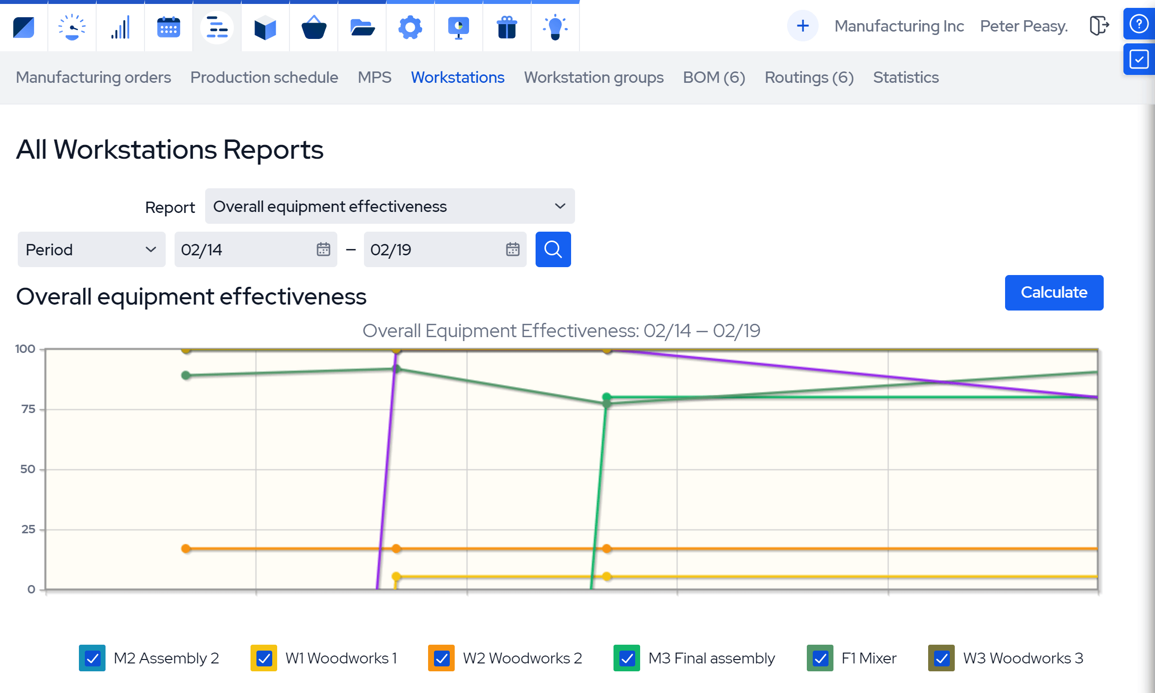
In MRPeasy, data capture happens at the operation. Operators report materials and operations as they work, so costs update in real time instead of at month’s end. The same transaction carries both lot and serial numbers, so the KPI and the traceability record come from one place.
Planned values lock when the order starts, not when it’s created. That’s the moving denominator from KPI #2 solved at the system level. You get planned versus actual duration and cost, order by order. You don’t get OEE, only the transactions it’s built from.
Extending the picture with Power BI
Trending across periods, blending production with financials, building a rollup nobody shipped as standard: that’s the Power BI integration’s job. MRPeasy pushes eleven tables into Power BI Service with the relationships already configured.
The window is the last twelve months, and the upload is manual, each push overwriting the last rather than syncing live. Power BI is where you analyze the operation, not where you watch it.
BI tools chart whatever you feed them. Capture at the event is what makes the chart worth building, and what separates a dashboard people rely on from one they quietly stop opening.
Frequently asked questions (FAQ)
Manufacturing KPIs help identify where time, materials, labor, and equipment capacity are being lost. Metrics such as OEE, throughput, downtime, and first pass yield can reveal bottlenecks and recurring problems. Tracking these KPIs over time allows manufacturers to measure whether process improvements are actually increasing production efficiency.
Overall Equipment Effectiveness (OEE) measures how effectively manufacturing equipment is used based on availability, performance, and quality. It is calculated by multiplying these three factors together. OEE matters because it helps manufacturers identify losses caused by downtime, slow production, and defects.
Cycle time measures how long it takes to complete a specific production process or manufacture a unit once work begins. Lead time measures the total time from the start of a request or order until it is completed or delivered. Cycle time is therefore one component that can influence overall manufacturing lead time.
Manufacturing KPIs should be updated often enough to support the decisions they influence. Shop-floor metrics such as downtime, throughput, and quality may need daily or real-time tracking, while inventory turnover or cost per unit may be reviewed weekly or monthly. Small manufacturers should prioritize consistent, reliable data rather than trying to monitor every KPI in real time.
You might also like: The 8 Wastes of Lean Manufacturing
Get manufacturing know-how delivered to your inbox!